Potential Flow Past a Cylinder in a Channel: OpenFOAM Verification
Key result: the potentialFoam solution of the flow past a cylinder matches the analytical solution for a cylinder between two walls to $0.9\%$ on average, and to $0.3\%$ next to the cylinder. The peak speed is twice the free-stream speed, at the top of the cylinder. The $5.4\%$ average departure from the classical unbounded solution comes from the walls, not from the solver.
SUMMARY
The inviscid, irrotational (potential) flow past a circular cylinder was computed with potentialFoam, the potential flow solver of the computational fluid dynamics (CFD) toolbox OpenFOAM [ref. 1], and compared with two analytical solutions. The cylinder, of radius $R = 0.5\,\mathrm{m}$, sits in a uniform stream $U_\infty = 1\,\mathrm{m/s}$ between two symmetry planes $4\,\mathrm{m}$ apart; only the upper half of the flow is computed, on a structured mesh of 2000 cells. The solution takes $0.04\,\mathrm{s}$. The speed next to the cylinder follows the expected $2 U_\infty \sin\theta$ distribution, with a peak of $2.011\,U_\infty$ at the top of the cylinder. Compared with the classical solution for a cylinder in an unbounded stream [ref. 2], the velocity differs by $5.4\%$ on average and $9.1\%$ at most. This difference is the blockage of the channel: the cylinder fills a quarter of its height, and the flow speeds up to pass it. Compared with the analytical solution for a cylinder between two walls, built by the method of images [ref. 3], the difference falls to $0.9\%$ on average, $0.3\%$ within $0.1\,\mathrm{m}$ of the cylinder, and $1.1\%$ at most there. The velocity field is verified; the approximate pressure field written by potentialFoam, on the other hand, falls well short of Bernoulli's equation on this mesh, and the pressure on the cylinder should be taken from the velocity.
INTRODUCTION
The flow past a circular cylinder is the textbook case of external aerodynamics: it has a closed-form solution in the ideal (inviscid) limit, and it is the first test of any flow solver. In the potential flow model the fluid has no viscosity and no rotation, so the velocity derives from a potential $\Phi$ that satisfies Laplace's equation. The model ignores the boundary layer and the wake, but it gives the speed and the pressure around the front of a body well, and it is used in practice to start viscous simulations from a realistic flow field instead of from rest.
The question of this study is how well potentialFoam reproduces the analytical solution, and what limits its accuracy. Following a rigorous sequence of steps, defining the geometry, the mesh (a discretisation of the domain), the boundary conditions and the solver settings, the study computes the velocity, pressure and stream function fields, and compares them with the analytical solutions for an unbounded stream and for a stream between two walls.
METHODOLOGY
The fluid is incompressible, inviscid and irrotational. The velocity derives from a potential, $\mathbf{U} = \nabla \Phi$, and mass conservation, $\nabla \cdot \mathbf{U} = 0$, gives Laplace's equation:
$$ \begin{equation} \nabla^2 \Phi = 0. \end{equation} $$
potentialFoam solves equation $(1)$ by the finite volume method, then reconstructs the velocity from the face fluxes. It can also estimate the kinematic pressure $p$ (pressure divided by density, in $\mathrm{m^2/s^2}$) from a Poisson equation; this pressure is meant as a starting field for a viscous solver.
Figure 1 represents the general setup of the problem. The domain is the rectangle $-2 \le x \le 2\,\mathrm{m}$, $0 \le y \le 2\,\mathrm{m}$, minus the half-disc of the cylinder, of radius $R = 0.5\,\mathrm{m}$, centred at the origin. The flow is symmetric about the axis $y = 0$, so only the upper half is computed. The flow is two-dimensional: the mesh is one cell thick in $z$, and the front and back planes are of the empty type.
The boundary conditions are the following. On the inlet ($x = -2\,\mathrm{m}$), the velocity is uniform, $\mathbf{U} = (U_\infty, 0, 0)$ with $U_\infty = 1\,\mathrm{m/s}$. On the outlet ($x = 2\,\mathrm{m}$), the pressure is fixed, $p = 0$, and the velocity has a zero normal gradient. The axis ($y = 0$) and the top boundary ($y = 2\,\mathrm{m}$) are symmetry planes: the flow cannot cross them, but slides freely along them. The top boundary therefore acts as a frictionless wall, and the full flow is that of a cylinder centred in a channel of height $2h = 4\,\mathrm{m}$. The cylinder surface is a slip wall (symmetry type), as required by an inviscid flow.
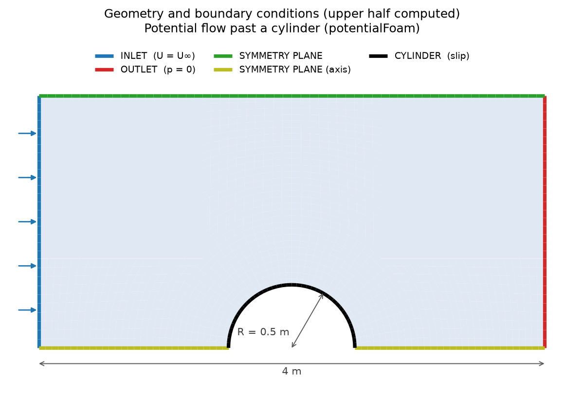
FIGURE 1. Geometry and boundary conditions. Only the upper half of the flow is computed; the axis and the top boundary are symmetry planes, and the cylinder is a slip wall.
Which analytical solution?
For a cylinder in an unbounded uniform stream, the velocity in polar coordinates $(r, \theta)$ is [ref. 2]
$$ \begin{equation} u_r = U_\infty \left(1 - \frac{R^2}{r^2}\right) \cos\theta, \qquad u_\theta = -U_\infty \left(1 + \frac{R^2}{r^2}\right) \sin\theta. \end{equation} $$
On the surface, $r = R$, the speed is $2 U_\infty |\sin\theta|$: it is zero at the two stagnation points, in front of and behind the cylinder, and reaches twice the free-stream speed at the top. This solution is written by the case itself, as the field UA, together with the relative error $|\mathbf{U} - \mathbf{U}_A| / |\mathbf{U}_A|$ in each cell.
The computed flow, however, is not unbounded: the top symmetry plane is only $4 R$ from the centre of the cylinder, and the cylinder fills a quarter of the channel height. The flow between the cylinder and the wall must speed up to carry the same flow rate. The method of images accounts for the walls [ref. 3]: a doublet (the singularity that turns a uniform stream into the flow past a cylinder) is mirrored in both walls, then the images in their images, which gives an infinite row of doublets spaced $2h$ apart along $y$. Its complex potential, with $z = x + iy$ and $k = \pi / 2h$, is
$$ \begin{equation} W(z) = U_\infty \left[ z + a^2 k \coth(k z) \right], \qquad u - i v = \frac{dW}{dz} = U_\infty \left[ 1 - \frac{a^2 k^2}{\sinh^2(k z)} \right]. \end{equation} $$
The doublet strength $a^2$ is set so that the front stagnation point lies on the cylinder, $x = -R$: $a^2 = \sinh^2(kR) / k^2 = 0.2631\,\mathrm{m^2}$, against $R^2 = 0.25\,\mathrm{m^2}$ in an unbounded stream. With this strength, the dividing streamline $\psi = 0$ crosses the vertical axis at $y = 0.4995\,\mathrm{m}$, so it follows the cylinder to within $0.1\%$. This solution is used here as the confined reference.
Mesh. The mesh was generated with blockMesh, from 10 hexahedral blocks arranged as an O-grid around the cylinder and a Cartesian grid outside it. It has 2000 hexahedral cells, one cell thick (figure 2). The ring $0.5 \le r \le 1\,\mathrm{m}$ around the cylinder has 10 cells across and 40 cells along the half-circumference, so each cell spans $0.05\,\mathrm{m}$ radially and $4.5^\circ$ around the cylinder; the cell centres next to the wall are at $r = 0.525\,\mathrm{m}$. The cylinder is represented by 40 flat faces, whose centres lie at $R \cos(2.25^\circ) = 0.4996\,\mathrm{m}$. The mesh passes all the checks of checkMesh: the largest aspect ratio is 1.98, the non-orthogonality is $10.1^\circ$ on average and $41.3^\circ$ at most (at the corners of the O-grid), and the largest skewness is 0.42.
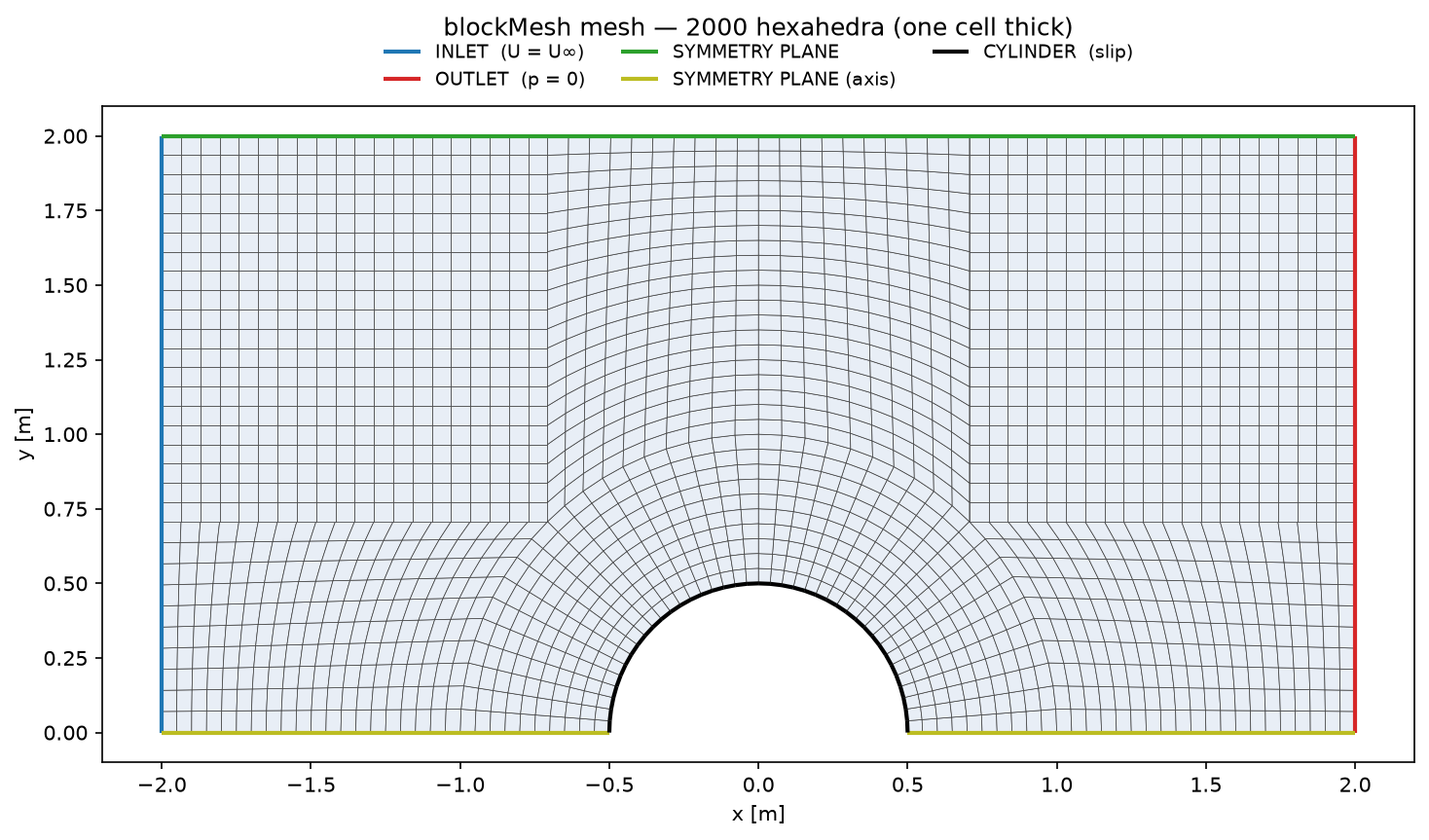
FIGURE 2. Mesh, 2000 hexahedra one cell thick, with an O-grid ring around the cylinder.
Solver. Equation $(1)$ is solved with a geometric-algebraic multigrid solver (GAMG) to a tolerance of $10^{-6}$, with three non-orthogonal correctors to account for the skewed cells of the O-grid. The gradients use least squares, and the Laplacian uses linear interpolation with a non-orthogonal correction. The analysis was run with OpenFOAM v2506 in its official Docker image.
RESULTS
The four solutions of the potential reduce the residual from $1$ to $3.4 \times 10^{-6}$. The continuity error is $1.4 \times 10^{-4}$ and the difference between the velocity reconstructed in the cells and the face fluxes is $1.2 \times 10^{-5}$, so the solution is converged and conserves mass. The solver takes $0.04\,\mathrm{s}$.
Figure 3 shows the velocity magnitude, mirrored about the axis. The flow slows down to nearly zero in front of and behind the cylinder, at the two stagnation points, and speeds up over the top and the bottom. The largest speed is in the cells next to the top of the cylinder: $|\mathbf{U}| = 2.011\,U_\infty$. The flow is symmetric front to back, as expected without viscosity: a potential flow has no wake.
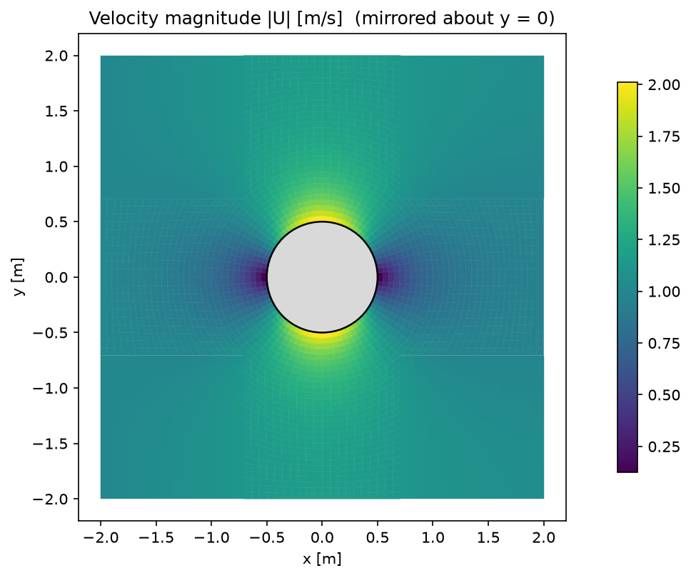
FIGURE 3. Velocity magnitude ($\mathrm{m/s}$), mirrored about $y = 0$.
Figure 4 compares the speed in the cells next to the cylinder with the analytical solutions. The computed points follow the $\sin\theta$ shape from the front stagnation point to the rear one. They lie above the unbounded solution evaluated at the same radius ($1.904\,U_\infty$ at the top): the walls speed the flow up. The confined solution of equation $(3)$ gives $2.009\,U_\infty$ at the top cell, against $2.011\,U_\infty$ computed, a difference of $0.1\%$. That the computed points also lie on the unbounded curve at $r = R$ is a coincidence: the speed-up due to the walls ($+5.4\%$) and the decrease of speed from the surface to the first cell centres ($-5\%$) nearly cancel.
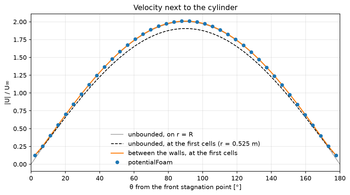
FIGURE 4. Speed next to the cylinder, $|\mathbf{U}|/U_\infty$, against the angle from the front stagnation point. Points: potentialFoam, at the cell centres ($r = 0.525\,\mathrm{m}$). Dashed: unbounded solution at the same radius. Grey: unbounded solution on the surface, $2|\sin\theta|$. Orange: solution between the walls, equation $(3)$, at the cell centres.
Figure 5 shows the relative difference with the unbounded solution. It is $5.4\%$ on average and $9.1\%$ at most. It is not largest at the cylinder, where the mesh is the most curved, but on the top wall above it, at $(0, 1.97)\,\mathrm{m}$: there the computed speed is $1.161\,U_\infty$, against $1.064\,U_\infty$ for the unbounded flow. The confined solution gives $1.162\,U_\infty$ at this point. The pattern of the figure is thus the signature of the walls, not of a numerical error. The thin lines along the block boundaries of the mesh are small jumps of the error (below $2\%$) where the cell size changes abruptly.
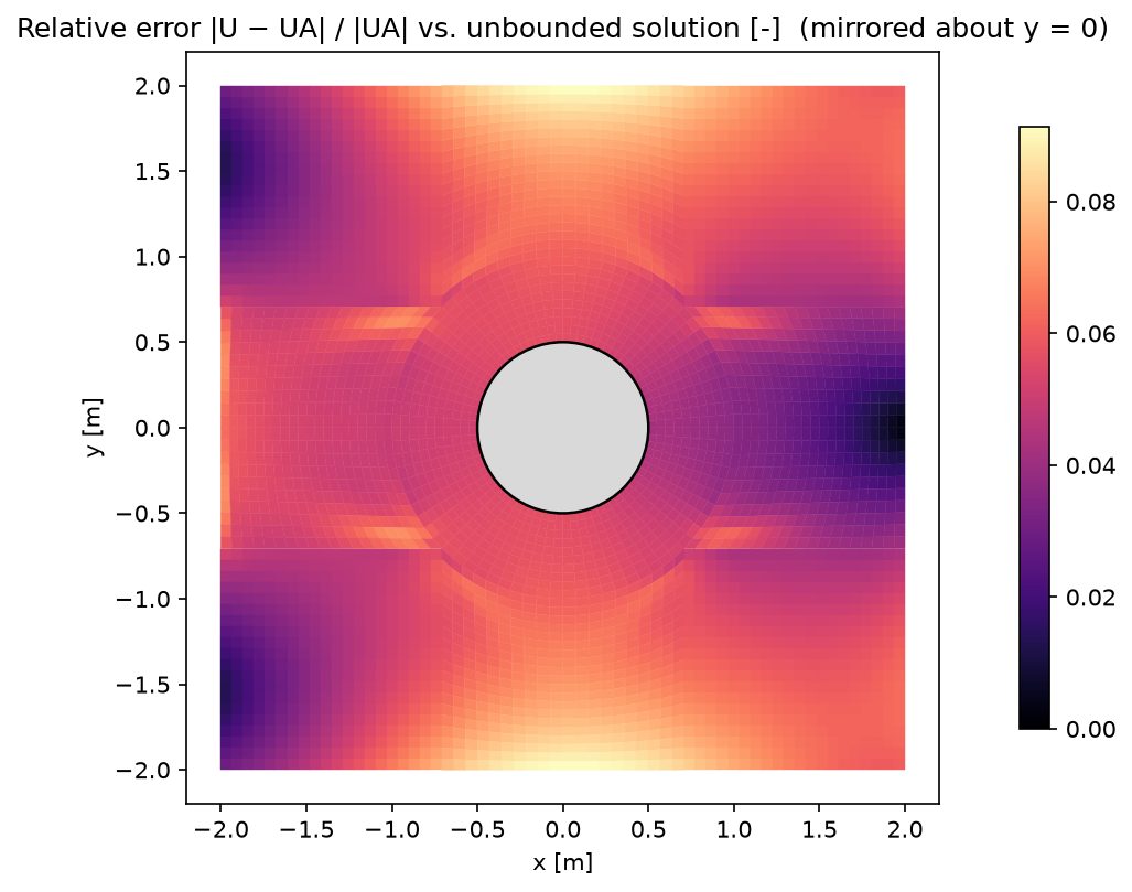
FIGURE 5. Relative difference with the unbounded solution, $|\mathbf{U} - \mathbf{U}_A|/|\mathbf{U}_A|$, mirrored about $y = 0$.
Measured against the confined solution of equation $(3)$, the difference falls to $0.9\%$ on average over the domain. Within $0.1\,\mathrm{m}$ of the cylinder ($r < 0.6\,\mathrm{m}$) it is $0.3\%$ on average and $1.1\%$ at most. The largest difference, $4.7\%$, is in the first column of cells at the inlet: the computation imposes a uniform velocity at $x = -2\,\mathrm{m}$, while the confined solution is still slowed down there by the cylinder ($0.97\,U_\infty$ on the axis). Outside the first and last columns of cells, the difference stays below $2.9\%$. Figure 6 shows this difference on the same scale as figure 5: the pattern of the walls is gone, and what remains is concentrated at the inlet and along the block boundaries of the mesh, where the cell size changes.
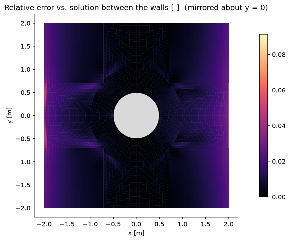
FIGURE 6. Relative difference with the solution between the walls, equation $(3)$, mirrored about $y = 0$, on the same scale as figure 5.
Figure 7 shows the streamlines. Near the cylinder they coincide with those of the unbounded solution. Further out, the computed streamlines are flatter, held by the top wall, which is itself a streamline. The small kinks at $x \approx 0.7\,\mathrm{m}$ are where the O-grid meets the Cartesian blocks.
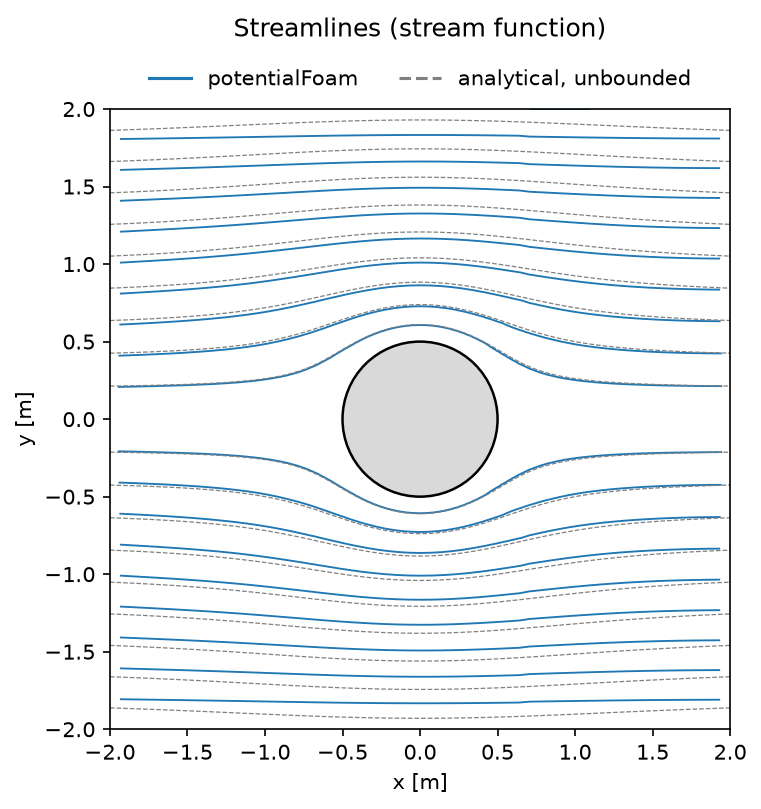
FIGURE 7. Streamlines (contours of the stream function). Solid: potentialFoam. Dashed: unbounded solution.
Figure 8 shows the approximate pressure written by potentialFoam, relative to the outlet. It has the right pattern: high at the two stagnation points and low over the top and the bottom of the cylinder. Its magnitude is not right, however. In a potential flow the pressure follows from the velocity by Bernoulli's equation, $p + |\mathbf{U}|^2/2 = \text{constant}$. Between the front stagnation cell and the top cell, the computed velocity gives a pressure drop of $2.01\,\mathrm{m^2/s^2}$, while the potentialFoam pressure drops by only $1.12\,\mathrm{m^2/s^2}$. At the front stagnation point it is $0.38\,\mathrm{m^2/s^2}$, against $0.49\,\mathrm{m^2/s^2}$ from Bernoulli. This pressure is only meant to start a viscous computation; for the loads on the body, the pressure must be taken from the velocity, through the pressure coefficient
$$ \begin{equation} C_p = \frac{p - p_\infty}{\tfrac{1}{2} U_\infty^2} = 1 - \frac{|\mathbf{U}|^2}{U_\infty^2}, \end{equation} $$
which gives $C_p = -3.05$ at the top cell (from $-3$ on the surface of a cylinder in an unbounded stream, to $-3.44$ on the surface between these walls).
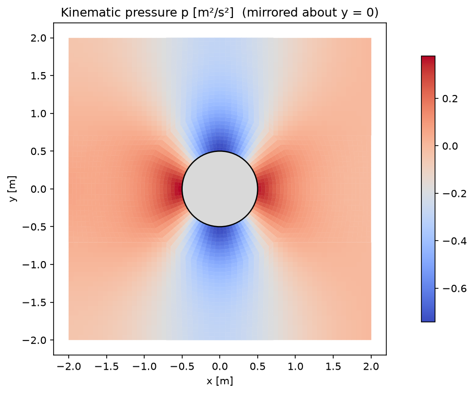
FIGURE 8. Approximate kinematic pressure $p$ ($\mathrm{m^2/s^2}$) written by potentialFoam, mirrored about $y = 0$.
| Quantity | potentialFoam | Unbounded | Confined |
|---|---|---|---|
| Speed at the top cell, $r = 0.525\,\mathrm{m}$ ($U_\infty$) | $2.011$ | $1.904$ | $2.009$ |
| Speed on the top wall, $(0, 1.97)\,\mathrm{m}$ ($U_\infty$) | $1.161$ | $1.064$ | $1.162$ |
| Mean relative difference, whole domain | $5.4\%$ | $0.9\%$ | |
| Mean relative difference, $r < 0.6\,\mathrm{m}$ | $5.2\%$ | $0.3\%$ | |
| Max relative difference, $r < 0.6\,\mathrm{m}$ | $5.7\%$ | $1.1\%$ | |
| Max relative difference, whole domain | $9.1\%$ | $4.7\%$ (inlet) | |
| $C_p$ at the top cell (Bernoulli) | $-3.05$ | $-2.63$ | $-3.04$ |
CONCLUSION
The potential flow past a circular cylinder was computed with potentialFoam on a 2000-cell structured mesh, with the goal of verifying the solver against analytical solutions and identifying what limits its accuracy. The solution converges, conserves mass, and reproduces the expected flow: two stagnation points, a peak speed of twice the free stream at the top of the cylinder, and no wake. It departs from the textbook unbounded solution by $5.4\%$ on average, but this departure is physical: the symmetry plane at $y = 2\,\mathrm{m}$ is a wall, and the cylinder blocks a quarter of the channel. Against the analytical solution of a cylinder between two walls, built by the method of images, the difference falls to $0.9\%$ on average and $0.3\%$ next to the cylinder. On this coarse mesh, the discretisation error is thus an order of magnitude smaller than the effect of the domain size.
Two practical lessons follow. First, a verification against an analytical solution must use the same problem: here, comparing with the unbounded solution would have suggested a $5\%$ solver error that does not exist. To compare with the unbounded flow, the walls must be moved away; the blockage effect decreases roughly as the square of the blockage ratio, so a channel ten times the diameter would bring it below $1\%$. Second, the pressure written by potentialFoam is only a starting field: on this mesh it underestimates the pressure differences by about $45\%$, and the surface pressure must be computed from the velocity with Bernoulli's equation. Since a real cylinder flow separates and sheds a wake, the potential solution describes the front of the cylinder well, but not the rear; it is the starting point for a viscous computation, not a substitute for it.
REFERENCES
- OpenFOAM, version v2506, solver potentialFoam.
- G. K. Batchelor, An Introduction to Fluid Dynamics, Cambridge University Press, 1967, section 6.6.
- L. M. Milne-Thomson, Theoretical Hydrodynamics, 5th edition, Macmillan, 1968, chapter 6 (method of images).